This is the second (and final) part of my series on ACME and pyacmegraph.
For the 1st post, see here: ACME and pyacmegraph – part 1 / 2
In this post I will detail pyacmegraph features and functioning.
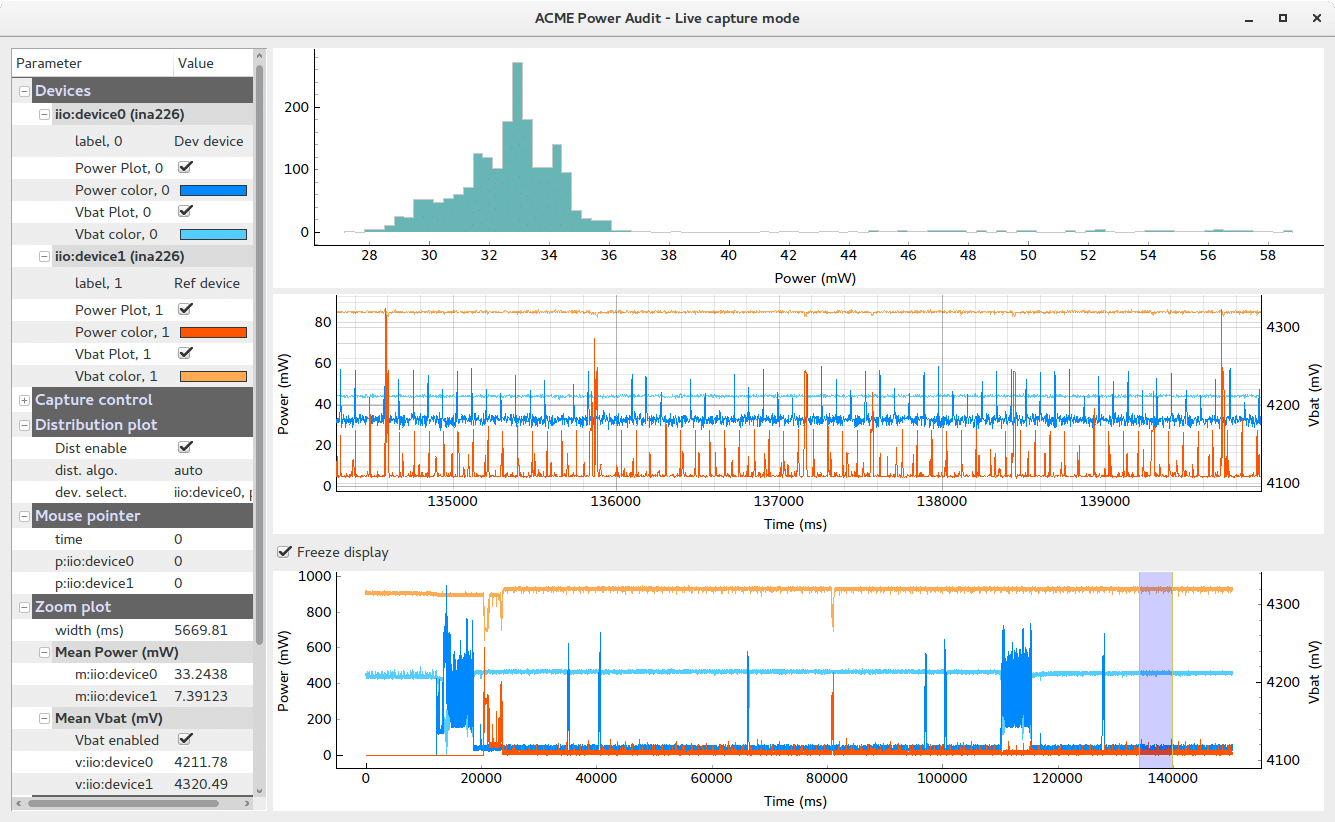
Here is a capture of pyacmegraph in action:

Features
Here is a recap on pyacmegraph features:
- auto-detect connected ACME probes and their Rshunt, setup the probes and capture data from probes
- compute and display Power consumption and Vbat with multiple zoom capabilities
- real-time statistics: mean Power, mean Vbat, distribution graph on a selected channel
- support any number of probes on an ACME cape
- save captured data for later offline visualization with pyacmegraph (view mode)
- save data as text or image
- re-use a saved data file UI settings for a fresh run (like device names, enabled plots, colors, Rshunts, …)
- can display Ishunt instead of power
- can force the use of a fixed Vbat value instead of the Vbat data captured from ACME probe
- control ACME probes power switch
Starting pyacmegraph in capture mode
Upon startup, pyacmegraph will try to connect to an IIO device using libiio. As such we can indicate an IP address for an IIO device using the --ip command-line parameter:
pyacmegraph.py --ip my-acme-ipaddress.local
or use the IIOD_REMOTE libiio environment variable:
IIOD_REMOTE=my-acme-ipaddress.local pyacmegraph.py
(this works whether ACME is connected to the local network or directly through USB – functional since Yocto pre-release b1 found here: https://github.com/baylibre-acme/ACME/releases)
Once connected, pyacmgraph will enumerate the various connected probes, setup them for optimal performances and will start capturing data. This is the default mode.
Note that you can get more information on this enumeration process by enabling the 1st verbose level with the -v command-line parameter.
pyacmegraph UI and features walk-through
Command line options
Here are the currently supported command-line options:
$ pyacmegraph.py --help

usage: pyacmegraph.py [-h] [--load file] [--template file] [--inttime [value]]

[--oversmplrt value] [--norelatime] [--ip IP]

[--shunts SHUNTS] [--vbat VBAT] [--ishunt]

[--forcevshuntscale [scale]] [--verbose]
(…)
More details are provided in the help command, and below are some additional information on these features.
Configuration pane
pyacmegraph re-uses many features from the pyqtgraph library. This includes the configuration pane, used for reporting static or live information and configuration. It is visible on the left of the screen and contains the following categories:
- Devices: editable values for
- device name,
- plots color (for each device we can plot the Power and/or Vbat),
- enable / disable: which plots to display
- Capture control: capture-related settings (only available in capture mode)
- Re-init buffers button: click to reset the capture buffers (and lose all captured data)
- Power-switches: if you connect some ACME probes embedding a power switch (like the Jack or USB probes) and use an ACME SW release supporting XMLRPC for controlling the probes (starting from Yocto b1 pre-release), you will be able to directly control the probe power-switch from these check-boxes
- plot-rate: time interval for refreshing the UI (re-plot graphs) – edit-able
- Rshunts: the shunt resistors values used for converting Vshunt to Ishunt or Power – edit-able
- Buffer period stats: per-device information on last captured buffer length
- Samples per second: per-devide information on samples captured per second (mean on 10 last captured buffers)
- oversampling ratio: value used
- integration time: value used for all channels of all devices (time for ADC to make a sample)
- Distribution plot:
- Dist enable: enable / disable the distribution graph display (consumes more ressources when enabled)
- dist. algo: algorithm to apply for displaying the distribution (auto-select by default)
- dev. select.: device and channel selection for the distribution graph (displays the ditribution of a single (device, channel couple)
- Mouse pointer: displays the coordinates pointed to by the mouse pointer
- Zoom plot: displays information related to the zoom plot (middle graph window)
- width: time width displayed in the zoom graph
- Mean power: per device mean power computed over the zoom window range of values
- Mean Vbat: per device mean Vbat computed over the zoom windiw range of values
- File operations:
- Save to binary: saves captured data and UI settings into a .acme file (format specific to pyacmegraph)
- Save to text: export captured data to a text files using 1 file per device and one line per time-stamp with values separated by comas
- Save to Picture: generates a PNG file from currently displayed graphs
Multiple zoom windows
On the right part of its UI, pyacmegraph displays 3 graphs arranged one below the other.

Here is their description from bottom to top:
- the bottom-most graph displays all the captured data (default setting). It includes a selection window. The content of this selection window is displayed in the graph located above:
- the middle graph is called the ‘zoom plot‘, and displays the content of the selection window of the bottom-most graph. Several metrics are computed on the data visible on this zoom plot (see left pane in ‘Zoom plot’ section). Also, one of the channel data visible in this zoom plot can be used to compute and display a distribution graph:
- the top-most graph, the ‘distribution plot‘ displays a distribution of the data for selected device channel, and corresponding to the range of data visible in the zoom plot. This distribution graph is disabled by default and can be enabled and configured using the configuration pane on the left.
Freezing displayed data
By default, all plot windows auto-update with the captured data, the bottom window shows the whole captured data and the zoom window the last 10s.
It is possible however, to enter in freeze mode, by enabling the Freeze display checkbox located between the bottom and zoom plots. In freeze mode data is still being captured and buffered but not displayed and the zoom and bottom plots can be scrolled and zoomed at will.
This mode makes easier to study a part of the live capture without interrupting it (it has not impact on the capture engine).
Offline and template features
As we could see it from the configuration pane, it is possible to save the captured data and UI settings into a .acme file.
.acme files can later be used in 2 ways:
First they can be re-opened with the --load command-line option. Example:
pyacmegraph.py --load savedfile.acme
This option runs pyacmegraph in offline mode: no connection to IIO devices are attempted and no data captured. Instead, the data and UI settings from the saved file are loaded and applied. This restores a working environment similar as when the data was saved. All the tool features are available. This is convenient to study captured data after the capture session, without the need to access to the capture device.
A second way of using a saved .acme file is with the --template command-line option. Ex:
pyacmegraph.py --ip my-acme-ip.local --template savedfile.acme
This option runs pyacmegraph in capture mode, connecting to an IIO device and capturing data from it. It ignores the data from the .acme file but loads and applies the UI settings from it. This is a convenient way of re-using a complete UI configuration (can contain custom device names, colors, shunt values, distribution graph settings, …).
Vbat related options
--vbat command-line option
There may be some cases where you don’t have access to a probe point for measuring Vbat, or are not interested in measuring it. The --vbat command-line options can help in this situation. It :
- disables the capture of the vbat value from the ACME probes, and
- forces a fixed value to be used as Vbat (this fixed value will be used for computing the device power)
(also note that disabling vbat capture increases the available bandwidth for capturing Vshunt)
--ishunt command-line option
If you are more interested in ploting the Ishunt value rather than the Power value, using the --ishunt command-line option does that.
Note that this option can be coupled to the --vbat one, hence disabling the vbat capture (makes sense if you don’t need it).
Probes configuration options
By default, pyacmegraph will setup ACME probes with optimal capture settings. However, it is possible to force different values:
inttime [VALUE]: (integration time) the time used at ADC level to capture one data sample. Use –inttime without value to get the list of discrete possible values.oversmplrt VALUE: (over-sampling rate) a multiply-factor used to increase sampling time (set to minimal value 1 by default).shunts VALUE1,VALUE2,...,VALUEn: IIO reports the default Rshunt value of the connected probes. However we can override these values by passing a series of Rshunt values to be used instead.
Conclusion
I hope that this overview of pyacmegraph answered most of your questions related to it and that its features will help you with your power management analysis!
If you have any questions, ideas or feedback, we will be happy to discuss on our #baylibre IRC channel on freenode.
Also, feel free to participate to this tool’s development, and to report bugs or ideas for improvement to the project Issues page: https://github.com/baylibre-acme/pyacmegraph/issues
pyacmegraph is available on GitHub here: https://github.com/baylibre-acme/pyacmegraph
For using this tool with ACME, you will need an IIO enabled ACME SW release, as found here https://github.com/baylibre-acme/ACME/releases (pre-built image with IIO)
Top-level ACME SW page on github: https://baylibre-acme.github.io
The ACME power measurement and remote access tool is developed by BayLibre. More info can be found on the product page. It is available for purchase online.